DataBricks is known as the Data Lake House. This is a combination of a data warehouse and data lake. This article will take a closer look at what this means in practice and how you can start your first experiments with DataBricks.{.preface}

You should know that the DataBricks platform is a spin-off of the Apache Spark project. As with many open source projects, the idea behind it was to combine open source technology with quality of life improvements.

DataBricks in particular obviously focuses on ease of use and a flat learning curve. Developers should resist the temptation to use an inexpensive, turnkey product instead of a  technically innovative system, especially for projects with a short lifespan.

Commissioning DataBricks

DataBricks is currently used exclusively in resources or implementations from cloud providers. At the time of writing this, the company at least supports the “Big Three”. Interestingly, in the [FAQ](https://www.databricks.com/product/faq) seen in **Figure 1**, they explicitly admit that they don’t currently provide the option of locally hosting the DataBricks system.

Fig. 1: If you want to host DataBricks locally, you’re out of luck.{.caption}

Interestingly, DataBricks has a close relationship with all three cloud providers. In many cases, you don’t have to pay separate AWS or cloud costs when purchasing a commercial DataBricks product. Instead, payment is made directly to DataBricks and the provider settles the costs.

For newcomers, there is the DataBricks Community Edition, a light version provided in collaboration with Amazon AWS. It’s completely free to use, but only allows 15 GB of data volume and is limited in terms of some convenience functions, scheduling (and the REST API). But this function should be enough for our first attempts. So let’s call up the [DataBricks Community Edition log-in page](https://community.cloud.databricks.com/login.html) in the browser of our choice. After clicking on the sign-up link, DataBricks takes you to the fully-fledged log-in portal, where you can register for a free 14-day trial of the platform’s full version. In order to use the Community Edition, you must first fully complete the registration process.

In the second step, be sure not to choose a cloud provider in the window shown in **Figure 2**. Instead, click the Get started with Community Edition link at the bottom to continue the registration process for the Community Edition.

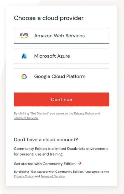
Fig. 2: Care is needed when activating the Community Edition.{.caption}

In the next step, you need to solve a captcha to identify yourself as a human user. The confirmation message seen in **Figure 3** is divided between the commercial and community edition. Don’t get anxious about the reference to the free trial phase.

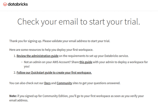
Fig. 3: Community Edition users also see this message.{.caption}

Entering a valid e-mail address is especially important. DataBricks will send a confirmation email. Clicking the link in the email lets you set a password. Then you’ll find yourself in the product’s start interface, [which can be activated later here](https://community.cloud.databricks.com/).

MYRIAD OF TOOLS & FRAMEWORKS

Tools, APIs & Frameworks

Learn more

Working through the Quickstart notebook

In many respects, commercial companies are interested in flattening the learning curve for potential customers. This can be seen in DataBrick’s guide. The Quickstart tutorial section is prominently placed on the homepage, offering the Start Tutorial link. Click it to command the web interface to change mode. Your efforts will be rewarded with a user interface similar to several Python notebook systems.

The visual similarities are no coincidence. DataBricks relies on the IPython engine in the background and is more or less compatible with standalone product versions. Creating the cluster is especially important here. Let me explain. The developer creates the intelligence needed to complete the machine learning task in the notebooks. But the actual execution of this intelligence requires computing power that normally far exceeds the available computing resources behind Schlomo Normaldevveloper’s browser window. Interestingly, DataBricks’ clusters are available in two versions. The all-purpose class is a classic cloud VM that (manually started and/or scheduled) is also available to a user rotation for collaboratively finishing battle tasks.

System number two is the job cluster. This is a dedicated cluster created for a batch task. It is automatically terminated after a successful or failed job processing. It’s important to note that the administrator isn’t able to keep a job cluster alive after the batch process finishes.

Be that as it may, in the next step, we place our mouse pointer on the far left to expand the menu. DataBricks offers two different operating modes by default. We want to choose Data Science and Engineering. In the next step, open the Compute menu. Here, we can manage the computing power sources in our account.

Activate the All-Purpose-Compute tab and click the Create Compute option to make a new cluster element. You can freely choose a name. I opted for SUSTest1. It’s important that several Runtime versions are available. In the following, we opt for the 7.3 LTS option (Scala 2.12, Spark 3.0.1). As free Community Edition users, we don’t have the option of choosing different cluster hardware sizes. Our system only ever has 15 GB of memory and deactivates after two hours of inactivity.

So, all you need to do to start the configuration process is click the Create Cluster button. Then, click the compute element again to switch to the overview table. This lists all of your account’s compute resources side-by-side. Generating the compute resources will take some time. To the far left of the table, as seen in **Figure 4**, there is a rotating circle symbol to show that our cluster is in progress.

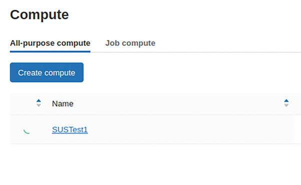
Fig. 4: If the circle is rotating, the cluster isn’t ready for combat yet.{.caption}

The start process can take up to five minutes. Once the work is done, a green tick symbol will appear, as seen in **Figure 5**. As a free version user, you cannot assume that your cluster is running ad perpetuum. If you notice strange behavior in the DataBricks, it makes sense to check the cluster status.

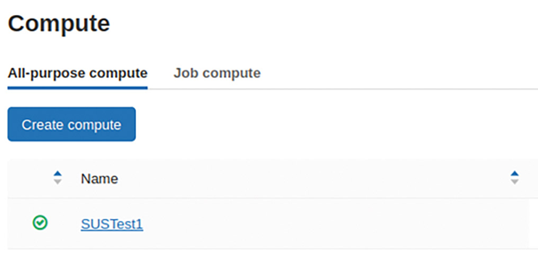
Fig. 5: The green tick mean it’s ready for action.{.caption}

Once our work is done, we can return to the notebook. The Connect option is available in the top right-hand corner. Click it and select the cluster to establish a connection. Then click 

the Run All icon next to it to instruct all commands in the notebook to execute. In the following, the system will execute commands in individual cells in real-time, as seen in **Figure 5**. Be sure to scroll down and view the results.

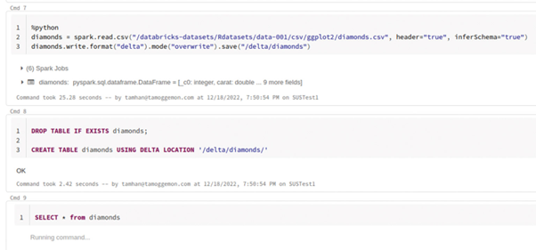
Fig. 6: The environment provides real-time information about operations performed

Focus on the cell.{.caption}

Due to the architectural decision to build DataBricks as a whole on IPython notebooks, we  must deliver the commands to be executed in the form of notebooks. Interestingly, the notebook as a whole can be kept in one programming language, while individual command cells can offer other languages. A foreign-language command element is created by clicking the respective language bubble, as shown in **Figure 7**.

Fig. 7: DataBricks allows the use of insular languages.{.caption}

Using the menu option File | Export | HTML, the DataBricks notebook can also be exported as an HTML file after its commands are successfully processed. The majority of the mark-up is lost, but the resulting file presents the results in a way that’s easier for management to understand and digest.

Alternatively, you can click the blue Publish button to generate a globally valid link that lets any user view the fully-fledged notebook. By default, these links stay valid for six months. Please note that publishing a new version invalidates all existing links.

Commercial version owners can also run their notebooks regularly like a cron job with the scheduling option. The user interface in **Figure 8** is used for this. Other job scheduling system users will feel right at home. However, be aware that this function requires a job cluster, which isn’t included and cannot be created in the free Community Edition at the time of writing this.

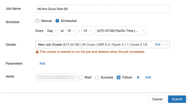
Fig. 8: DataBricks in scheduling mode.{.caption}

Last but not least, you can also stop the cluster using the menu at the top right. This is only a courtesy to the company for the Community Edition. But, it’s highly recommended for commercial use since it reduces overall costs.

Different data tables for optimizing performance

One of NoSQL databases’ basic characteristics is that in many cases, they soften the ACID criteria. The lower consistency quality is usually offset by a greatly reduced database administration effort. Sometimes, this results in impressive performance increases compared to a classic relational database. When working with DataBricks, we deal with a group of different table types that differ in terms of performance and data storage type.

The most important difference concerns external tables and managed tables. A managed table lives entirely in the DataBricks cluster. The development team understands this to mean that the database server handles management of the actual information and the provision of metadata and access features. There’s also the unmanaged or external table. This table represents a kind of “wrapper” around an external data source. Using this design pattern is recommended if you frequently use sample databases or information already available elsewhere in the system in an accessible form.

Since our sample from DataBricks is based on a diamond information set, using external tables is recommended. Redundant duplication of resources will only waste memory space in our cluster, without bringing any significant benefits here.

However, a careful look at the instructions created in the example notebook shows two different procedures. The first table is created with the following snippet:

```

DROP TABLE IF EXISTS diamonds;
CREATE TABLE diamonds
USING csv
OPTIONS (path "/databricks-datasets/Rdatasets/data-001/csv/ggplot2/diamonds.csv", header "true")
```

Besides the call to DROP TABLE, which is always needed to initialize the cluster, creating the new table uses standard SQL commands, more or less.We use _Using csv_ to tell the Runtime we want to use the CSV engine. If you scroll further down in the example, you’ll see that the table is created again, but in a two-stage process. In the first step, there’s now a Python island in the notebook that interacts with the diamond sample information in the URL /databricks-datasets/Rdatasets/data-001/csv/ggplot2/diamonds.csv according to the following:

```
%python
diamonds = spark.read.csv("/databricks-datasets/Rdatasets/data-001/csv/ggplot2/diamonds.csv", header="true", inferSchema="true")
diamonds.write.format("delta").mode("overwrite").save("/delta/diamonds")
```

The DataBricks development team provides aspiring data science experimenters with a dozen or so widely used sample datasets. These can be accessed directly from the DataBricks runtime using friendly URLs. Additional information about available data sources [can be found here](https://docs.databricks.com/dbfs/databricks-datasets.html).

In the second step, there’s a snippet of SQL code that delivers Using Delta instead of the previously used Using CSV. This instructs the DataBricks backend to animate the existing element with the Delta database engine.

```
DROP TABLE IF EXISTS diamonds;

CREATE TABLE diamonds USING DELTA LOCATION '/delta/diamonds/'
```

Delta is an open source database engine based on Apache Parquet. Its (https://github.com/delta-io/delta). Normally, it’s always preferable to use the Apache Spark table because it delivers better results in terms of both ACID criteria and performance, especially when large amounts of data need to be processed.

DataBricks is more – Focus on machine learning

Until now, we operated the DataBricks runtime in engineering mode. It’s optimized for the needs of ordinary data scientists who want to perform various types of analyses. But the user interface has a special mode specifically for machine learning (**Fig. 9** shows the mode switcher) that focuses on relevant functions.

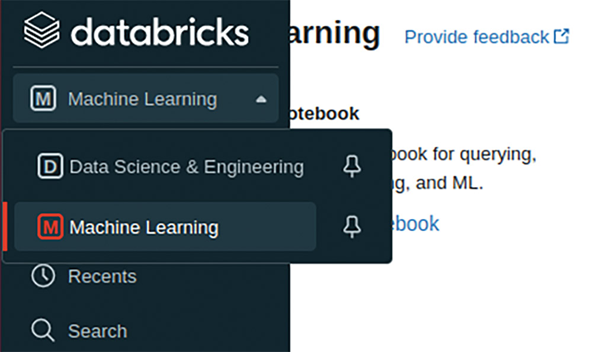
Fig. 9: This option lets you change the personality of the DataBricks interface.{.caption}

In principle, the workflow in **Figure 10** is always used. Anyone implementing this workflow in an in-house application will always work with the Auto-ML working environment sooner or later. In theory, this is available from version 9.1 at the end of Runtime, but it’s only really feature-complete when at least version 10.4 LTS ML is available on the cluster. But since this is one of the USPs of the DataBricks platform, we can assume that the product is under constant further development. It’s advised that you check if the cluster in question is running the product’s latest version. For data engineering, DataBricks also offers a dedicated tutorial in the Guide: Training section from the home screen. This makes it easier to get started. Click the Start guide option again to load the notebook for this tutorial as “to be edited”.

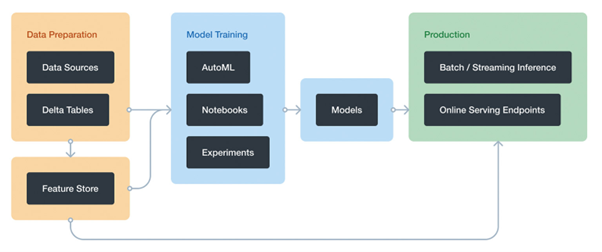
Fig. 10: If you want to use the ML functions in DataBricks, you should familiarize yourself with this workflow.{.caption}

Due to higher demands on the aforementioned required Data Bricks Runtime, you should switch to the Compute section and delete the previously created cluster. Then, click the Create Compute option again and delete the previously created cluster. Click the Create Compute option again and make sure to click the ML heading in the DataBricks Runtime Version field (see **Fig. 11**) in the first step.

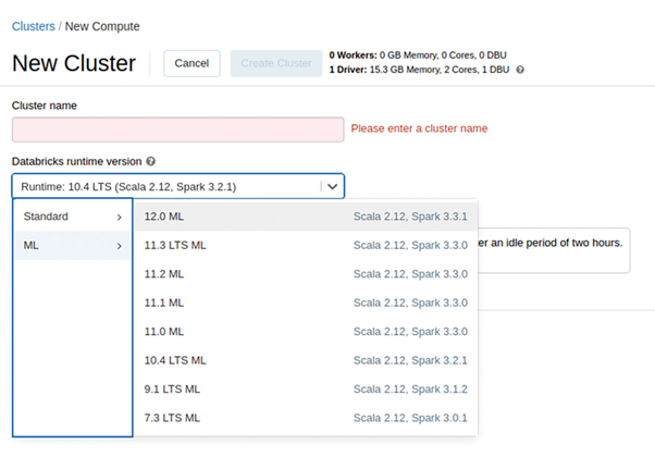
Fig. 11: ML-capable variants of the DataBricks runtime appear in a separate section in the backend.{.caption}

Just for fun, we’ll use the latest version 12.0 ML and name the cluster “SUSTestML”. It takes some time after clicking the Create Cluster button, since the cloud resources aren’t immediately provided.

During cluster generation, we can return to the notebook to get an overview of the elements. In the first step, we see the inclusion of the following libraries, abbreviated here. They are familiar to every Python developer:

```

import mlflow
import numpy as np
import pandas as pd
import sklearn.datasets
. . .
from hyperopt import fmin, tpe, hp, SparkTrials, Trials, STATUS_OK
. . .
```

In many respects, DataBricks is based on what ML developers are familiar with from working with standard Python scripts. Some libraries naturally have optimizations to make them run more efficiently on the DataBricks hardware. In general, however, a locally functioning Python script will continue to work without any problems after being moved to the DataBricks cluster. For the actual monitoring of the learning process, Data Bricks relies on MLFlow, which is available here [6].

For this reason, the rest of the notebook is standard ML code, although it’s elegantly integrated into the user interface. For example, there is a flyout in which the application provides information about various parameters that were created during the parameterization of the model:

```
with mlflow.start_run(run_name='gradient_boost') as run:
  model = sklearn.ensemble.GradientBoostingClassifier(random_state=0)
  model.fit(X_train, y_train)
  . . .
```

It’s also interesting to note that the results of the individual optimization runs are not only displayed in the user interface. The Python code that lives in the notebook can also access them programmatically. In this way, it can perform a kind of reflection to find the most suitable parameters and/or model architectures.

In the case of the example notebook provided by DataBricks, this is illustrated in the following snippet, which applies an SQL query to the results available in the mlflow.search_runs field:

“`

best_run = mlflow.search_runs(
  order_by=['metrics.test_auc DESC', 'start_time DESC'],
  max_results=10,
).iloc[0]
print('Best Run')
print('AUC: {}'.format(best_run["metrics.test_auc"]))
print('Num Estimators: {}'.format(best_run["params.n_estimators"]))
```

 AutoML, for the second time

The duality of control via the user interface and programmatic control also continues in the case of the AutoML library mentioned above. The user interface shown in Figure 12, which allows graphical parameterization of ML runs, is probably the most common marketing argument.

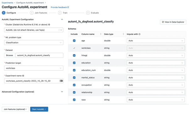
Fig. 12: AutoML allows the graphical configuration of modeling{.caption}

On the other hand, there is also a programmatic API that illustrates DataBricks in the form of a group of notebooks. Here we want to use the example notebook provided here [7], which we load into a browser window in the first step. Then click on the Import Notebook button at the top right and copy the URL to the clipboard. Next, open the menu of your DataBricks instance and select the Workspace File Users option. Next to your email address, there is a downward pointing arrow, which allows you to open a context menu. Select the import option there and then enter the URL to load the sample notebook into your DataBricks instance.

The actual body of the model couldn’t be any easier. In the first step, we mainly load test data, but we also create a schema element that informs the engine about the type or data type of the model information to be processed:

```

from pyspark.sql.types import DoubleType, StringType, StructType, StructField

schema = StructType([
  StructField("age", DoubleType(), False),
  . . .
  StructField("income", StringType(), False)
])
input_df = 
spark.read.format("csv").schema(schema).load("/databricks-datasets/adult/adult.data")
```
The actual classification run then also takes place with a single line:
```

from databricks import automl
summary = automl.classify(train_df, target_col="income", timeout_minutes=30)
```

If you want to carry out interference later, you can do this with both Pandas and Spark.

The multitool for ML professionals

Although there are hundreds of pages yet to be written about DataBricks, we’ll end our experiments with this brief overview. DataBricks is a tool that is completely focused on data scientists and machine learning experts and is not really suitable for beginners due to the very steep learning curve. Much like the infamous Squirrel Busters, DataBricks is a product that will find you when you need it.

References

[1] https://www.databricks.com/product/faq

[2] https://community.cloud.databricks.com/login.html

[3] https://community.cloud.databricks.com/

[4] https://docs.databricks.com/dbfs/databricks-datasets.html

[5] https://github.com/delta-io/delta

[6] https://www.mlflow.org/docs/latest/index.html

[7] https://docs.databricks.com/_static/notebooks/machine-learning/automl-classification-example.html